BZ Bread

by George Schils.

The SP 500 index as a random walk

Saturday, January 26, 2013

This brief blog post gives the results of some random walk studies applied to the stock market. In particular, a segment of S&P 500 stock market data is used for the analysis. The question is how does the stock market data compare to a random walk. To answer this question, the power spectrum is computed for a segment of stock market data. It is known that the power spectrum of a random walk decreases as the square of the frequency. The analysis that we do computes the power spectrum of a section of S&P 500 data, and compares the fall off over frequency with that of a random walk.

I am using the terminology "ramdom walk" to mean Brownian motion, and I may be a bit sloppy in using this term. Even though I use the term "random walk" in this post, a better term would be "Brownian motion".

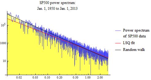
The first analysis that we do is for a time starting on January 1, 1950 and extending to January 1, 2013. The S&P 500 data over this period is used as input for the spectral analysis. The graphic below shows the result of the sample power spectrum, and also shows the ideal result for a pure random walk. The pure random walk has a power spectrum characteristic shown by the solid blue line. The sample power spectrum is shown as the jagged blue line. Because it is a sample spectrum, and not an average spectrum, one would expect it to be somewhat jittery, as we observe. It is observed that the sample power spectrum from the S&P 500 data closely follows the solid blue line for a pure random walk. Tentatively, this illustrates that the S&P 500 stock market data is very much that of a pure random walk. This is over the 63 year analysis period.

S&P 500 power spectrum over 63 year time period

In the above log-log plot, the solid blue line has a slope of -2. This means that the spectrum falls off at a rate proportional to the square of the frequency. This is the power spectrum of an ideal random walk. It is seen to correspond closely to the sample spectrum for the S&P 500 data.

The actual data used in this analysis is given in the graphic below. This is the value of the S&P 500 index over the period of 63 years, extending from the year 1950 to the year 2013.

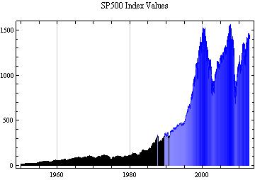
S&P 500 stock index since 1950

The basic result that stock market data follows a random walk appears not to depend strongly on the analysis period. We show results for two additional analysis periods. First, we look at data from 2005 to 2012. Secondly, we look at data from 2008 to 2012.

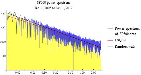
S&P 500 power spectrum from 2005 to 2012

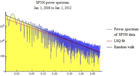
S&P 500 power spectrum from 2008 to 2012

A random walk is a lot like a drunk staggering down the street. This article discusses some humorous aspects of this phenomenon.

The red line in the above power spectrum graphs is a least squares fit. This red line is a naive least squares fit, and can be subject to various errors. The slopes that I get for this least squares fit range from about -1.5 to -1.75, whereas pure Brownian motion has a value of -2. If these slopes are correct, it would indicate fractional Brownian motion.

The results discussed above are tentative. There are many technical issues that are beyond the scope of this article.

Related references: 1, 2, 3, 4.

Update 2