
Back to Cfa research pages.
Examples of advanced versions of Cfa
We caution not to misinterpret these results. In some cases the results can change much depending on the numbers. We are not illustrating conclusions, but instead are illustrating techniques using our Cfa software. (Disclaimer)
There is quite a wide range of results on rent versus buy. The leveraging results depend very much on what the numbers are. This is one of the great powers and capabilities of Cfa: these sensitivies can be studied. The results on down payment are perhaps even more dramatic.
The calculations and results on this page were performed with the more advanced versions of Cfa. These more advanced versions allow single variables to be analyzed over a range of values, with corresponding results calculated and plotted. This is a very powerful analysis capability for graphical relationships and sensitivities to important variables can be studied.
Here is an example graph computed by Cfa of the first result shown below.
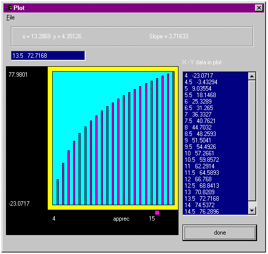
Calculation and graph of rate of return between
renting and buying as
a function of the apprecation rate of the home.
(Graph generated by more advanced versions of Cfa)
This graph is useful and portrays meaningful information. Moving the mouse over the data gives the data values as well as the slope (sensitivity). We admit though that higher quality graphics can be obtained by exporting this data into other tools designed specifically for graphics.
This graph is useful in the scientific sense because the data values themselves are displayed, and moving the mouse displays both the data values as well as the sensitivity. For example, at the point apprec = 5%, the sensitivity is about 21. This is the slope of the curve at this point. For every point the home appreciates (about this point), the rate of return goes up 21 points.
The "baseline" problem that we are working here uses the parameters for the problem discussed here. We will vary some of the parameters in this rent/buy problem, and we will portray the results graphically. (This graph is also shown above.)
..gvar percent-down 20.0
..gvar home-cost 160000
..gvar mortgage-interest 7.5
..gvar extra-payments -200
..gvar tax-bracket 25
..gvar tax-bracket-differential 5
..gvar apprec 5
..gvar selling-percent 7.0

..gvar rent-cost -650
..gvar rent-inc 0.00
..gvar account-rate 7
..gvar additional-deposit 0
The rate of return on the difference between buying and renting depends most dramatically on the home appreciation rate, as this graph shows. This is an interesting result. We coined the word "leveraging curve" since it shows the leveraging effect of buying a home.
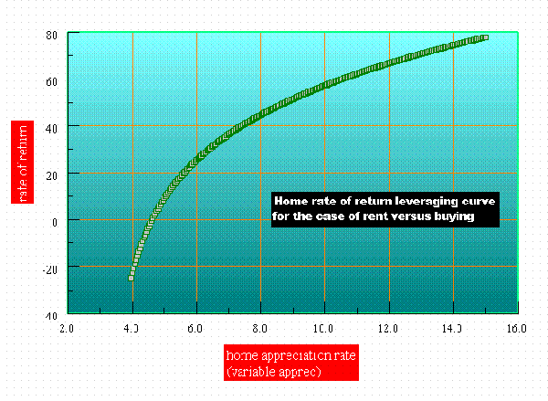
It may be hard to define what this rate of return on the difference between buying minus renting really means, and this is sometimes debated in textbooks. The PW may be a better measure for such a comparison, and this is discussed next.
PW calculation Now we vary the apprec rate from 4 to 15 % and we compute the PW of the difference between buying and renting (buy - rent). The discount rate for the PW calculation is 6% yearly. (The per period rate is this number divided by 12.) This only takes a minute or two in Cfa and the data is (it is easy to export such data)
4.000000        -4316.187735
4.500000        -1831.882235
5.000000        714.018762
5.500000        3323.015932
6.000000        5996.645867
6.500000        8736.481918
7.000000        11544.135063
7.500000        14421.254784
8.000000        17369.529976
8.500000        20390.689870
9.000000        23486.504980
9.500000        26658.788069
10.000000       29909.395141
10.500000       33240.226451
11.000000       36653.227547
11.500000       40150.390322
12.000000       43733.754107
12.500000       47405.406772
13.000000       51167.485867
13.500000       55022.179780
14.000000       58971.728925
14.500000       63018.426955
15.000000       67164.622009
This is plotted below.
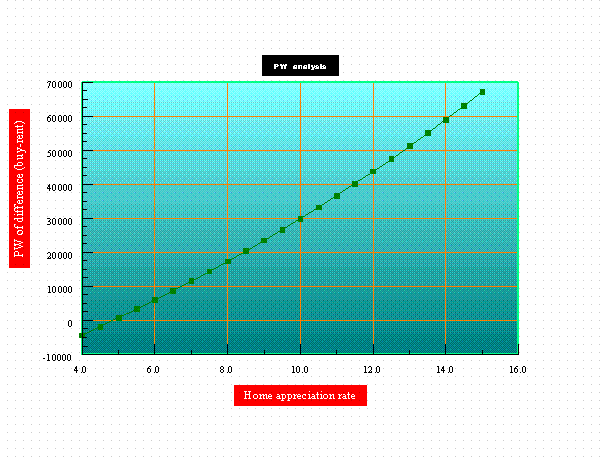
Plot of PW as a function of home appreciation rate
And of course, as we already know, we can do very well if the home appreciates at a high rate. The calculations here show this exact quantititative relationship, and can be performed in only a few minutes using the advanced versions of Cfa.
We use the same set of numbers as listed above, but this time we will vary the tax bracket from 15% to 45%. The calculated PW (discounted at 6%) on the difference between buying minus renting is given by this data:
15.000000       -1107.882959
16.000000       -925.692787
17.000000       -743.502615
18.000000       -561.312443
19.000000       -379.122270
20.000000       -196.932098
21.000000       -14.741926
22.000000       167.448246
23.000000       349.638418
24.000000       531.828590
25.000000       714.018762
26.000000       896.208934
27.000000       1078.399106
28.000000       1260.589278
29.000000       1442.779450
30.000000       1624.969622
31.000000       1807.159794
32.000000       1989.349966
33.000000       2171.540138
34.000000       2353.730310
35.000000       2535.920482
36.000000       2718.110654
37.000000       2900.300826
38.000000       3082.490998
39.000000       3264.681170
40.000000       3446.871342
41.000000       3629.061514
42.000000       3811.251686
43.000000       3993.441858
44.000000       4175.632030
45.000000       4357.822202
This data is plotted below.
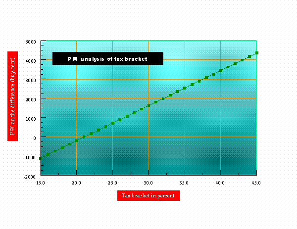
PW of buying minus renting as a function of tax bracket
This data is a straight line with a slope of 182.19. For every point that the tax bracket goes up, the PW (on the difference) goes up 182.19. Of course in the higher tax brackets we are better off buying because this increases the home mortgage interest deduction, and further we are worse off in the case of renting because we pay more tax in the interest earned on the CD. We have demonstrated the exact quantitative dependence on the tax bracket.
Also notice that there is a breakeven tax bracket (around 21%) where buying and renting will have about equal PW (when discounted at 6%). Of couse this breakeven value depends on what numbers we choose, and this is NOT a general conclusion. Cfa calculates the breakeven tax bracket to be 21.1% indeed, a very easy calculation.
We vary the percent down payment for the mortgage from 1% to 30% and we calculate both the PW and rate of return on the difference between buying minus renting. Again the results are very interesting.
PW. The PW (discounted at 6%) as a function of the percent down payment is computed as
1.000000        -511.154415
2.000000        -446.671617
3.000000        -382.188818
4.000000        -317.706019
5.000000        -253.223220
6.000000        -188.740421
7.000000        -124.257623
8.000000        -59.774824
9.000000        4.707975
10.000000       69.190774
11.000000       133.673573
12.000000       198.156371
13.000000       262.639170
14.000000       327.121969
15.000000       391.604768
16.000000       456.087567
17.000000       520.570365
18.000000       585.053164
19.000000       649.535963
20.000000       714.018762
21.000000       778.501561
22.000000       842.984359
23.000000       907.467158
24.000000       971.949957
25.000000       1036.432756
26.000000       1100.915554
27.000000       1165.398353
28.000000       1229.881152
29.000000       1294.363951
30.000000       1358.846750
This PW series of data is plotted below.
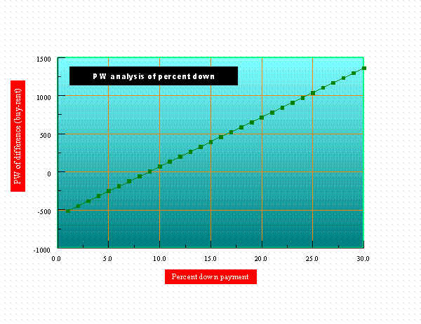
PW for buy-rent as a function of percent down payment
This is a straight line with slope 64.48. We note that the results on down payment can depend very much on what the numbers are. Try it with your own numbers.
Rate of return. Another interesting calculation is the rate of return on the difference as a function of the percent down payment. The data from this calculation is:
1.000000        5.007884
2.000000        5.107565
3.000000        5.213279
4.000000        5.325593
5.000000        5.445144
6.000000        5.572659
7.000000        5.708961
8.000000        5.854995
9.000000        6.011844
10.000000       6.180759
11.000000       6.363194
12.000000       6.560846
13.000000       6.775709
14.000000       7.010143
15.000000       7.266963
16.000000       7.549557
17.000000       7.862030
18.000000       8.209423
19.000000       8.597979
20.000000       9.035544
21.000000       9.532113
22.000000       10.100628
23.000000       10.758177
24.000000       11.527816
25.000000       12.441491
26.000000       13.544894
27.000000       14.906004
28.000000       16.631202
29.000000       18.898605
30.000000       22.036643
This data is plotted below.
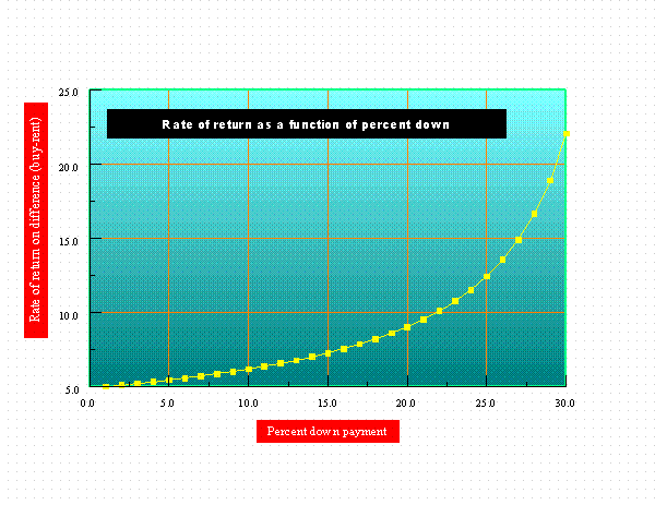
Rate of return on difference between buying minus renting as
a function of percent down
These results are very interesting.
HTML revision number: $Revision: 1.5 $